Install LowMACA
source("http://bioconductor.org/biocLite.R")
biocLite("LowMACA")
External Resources
LowMACA relies on three external resources to work properly.
- Clustal Omega, our trusted aligner
- Ghostscript, a postscript interpreter needed to draw logo plots
- Protter, a tool for visualization of proteoforms and annotation of predicted sequences
Clustal Omega is a fast aligner that you can download from the link above. Be sure to have the word clustalo as an alias for the executable clustalomega (so don't forget to run chmod u+x clustalo ;) ).
- For Unix users (MacOS and Linux), we provide a sh script to download and install the program. If it doesn't work on your system, just follow the official readme
- For Windows user, simply download the binary zip file in clustal omega download page, unzip the folder and put the path to the folder in the PATH environment variable (like they show here)
Ghostscript is an interpreter of postscript language and a pdf reader that is used by the R library grImport.
- For Linux users, simply download the program from here and compile it
- For MacOS users there is a dmg installer here
- For Windows users, download the program from here and remember to run the command below at every new session of R or put the command in your .Renviron file
This command will set an R variable to use Ghostscript in the right way. Apparently, the R package that uses ghostscript (grImport) works on 32bit ghostscript version. So, download the 32bit version even if your Windows is 64bit.
# Needed only on Windows - run once per R session
# Adjust the path to match your installation of Ghostscript
> Sys.setenv(R_GSCMD = '"C:/Program Files/gs/gs9.05/bin/gswin32c.exe"')
Protter is a cool predictor and visualizer of protein sequence secondary structures. It's a web-based tool and doesn't require any special setting except from a internet connection.
Enjoy!
Use LowMACA
Using LowMACA is as easy as it gets! You don't need any particular knowledge of R to be able to play around and produce plots and statistics.
Create a LowMACA class object
- Find your target family of genes or pfam you want to know more about.
You can insert data as:- Gene names can be specified as Official Gene Symbol or Entrez ID. If you insert an alias for your favorite gene symbol, LowMACA will try to convert it to the official name if it is unambiguous.
- Pfam ids must be specified as PF#. Go to Pfam website for further specifications.
> library(LowMACA)
> myBelovedFolder <- "myLowMACAOutput"
> Genes <- c("ADNP","ALX1","ALX4","ARGFX","CDX4","CRX"
                        ,"CUX1","CUX2","DBX2","DLX5","DMBX1","DRGX"
                        ,"DUXA","ESX1","EVX2","HDX","HLX","HNF1A"
                        ,"HOXA1","HOXA2","HOXA3","HOXA5","HOXB1","HOXB3"
                        ,"HOXD3","ISL1","ISX","LHX8")
> Pfam <- "PF00046"
> lm <- newLowMACA(genes=Genes , pfam=Pfam , outputFolder=myBelovedFolder)
All Gene Symbols correct!
> str(lm)
Formal class 'LowMACA' [package "LowMACA"] with 4 slots
  ..@ arguments:List of 7
  .. ..$ genes      : NULL
  .. ..$ pfam       : chr "PF00046"
  .. ..$ input      :'data.frame':      29 obs. of  7 variables:
  .. .. ..$ Gene_Symbol   : Factor w/ 28 levels "ADNP","ALX1",..: 4 13 13 12 8 5 6 20 21 24 ...
  .. .. ..$ Pfam_ID       : Factor w/ 1 level "PF00046": 1 1 1 1 1 1 1 1 1 1 ...
  .. .. ..$ Entrez        : Factor w/ 28 levels "1046","1406",..: 26 27 27 28 16 1 2 7 8 11 ...
  .. .. ..$ Envelope_Start: int [1:29] 79 102 16 39 1169 174 40 144 192 189 ...
  .. .. ..$ Envelope_End  : int [1:29] 135 156 70 95 1225 230 96 200 248 245 ...
  .. .. ..$ UNIPROT       : Factor w/ 28 levels "ADNP_HUMAN","ALX1_HUMAN",..: 4 13 13 5 9 6 7 20 21 24 ...
  .. .. ..$ AMINO_SEQ     : chr [1:29] "HKERTSFTHQQYEELEALFSQTMFPDRNLQEKLALRLDLPESTVKVWFRNRRFKLKK" "RRCRTTYSASQLHTLIKAFMKNPYPGIDSREELAKEIGVPESRVQIWFQNRRSRL" "RRCRTKFTEEQLKILINTFNQKPYPGYATKQKLALEINTEESRIQIWFQNRRARH" "RRNRTTFTLQQLEALEAVFAQTHYPDVFTREELAMKINLTEARVQVWFQNRRAKWRK" ...
  .. ..$ mode       : chr "pfam"
  .. ..$ params     :List of 4
  .. .. ..$ mutation_type      : chr "missense"
  .. .. ..$ tumor_type         : chr "all"
  .. .. ..$ min_mutation_number: num 1
  .. .. ..$ density_bw         : num 0
  .. ..$ paths      :List of 2
  .. .. ..$ clustal_cmd  : chr "clustalo"
  .. .. ..$ output_folder: chr "myLowMACAOutput"
  .. ..$ parallelize:List of 2
  .. .. ..$ getMutations : logi FALSE
  .. .. ..$ makeAlignment: logi TRUE
  ..@ alignment: list()
  ..@ mutations: list()
  ..@ entropy  : list()
Now we have created a LowMACA object redirecting all the future output to a folder named "myLowMACAOutput". In this case, we want to analyze the homeodomain fold pfam (PF00046), considering 28 genes that belong to this clan. If we don't specify the pfam parameter, LowMACA proceeds to analyze the entire proteins passed by the genes parameter. Viceversa, if we don't specify the genes parameter, LowMACA looks for all the proteins that contain the specified pfam (or pfams if you wish) and analyze just the portion of the protein assigned to the domain.
- Change default parameters
As we can see, a LowMACA object is composed by four slots. The first slot is @arguments and is filled at the very creation of the object. It contains information as Uniprot name for the proteins associated to the gene (we map only canonical proteins, one per gene), the amino acid sequences, start and end of the selected domains and many default parameters that can be change to start the analysis.#See default parameters > lmParams(lm) $mutation_type [1] "missense" $tumor_type [1] "all" $min_mutation_number [1] 1 $density_bw [1] 0 #Change some parameters #Changing the minimum accepted number of mutations (we accept sequences even if they have no mutations) > lmParams(lm)$min_mutation_number <- 0 #Changing selected tumor type #Check the available tumor types in cBioPortal > showTumorType() [1] "laml" "acyc" "acc" "blca" "lgg" "brca" "cellline" "cesc" [9] "coadread" "esca" "escc" "gbm" "hnsc" "kich" "kirc" "kirp" [17] "lihc" "luad" "lusc" "dlbc" "mpnst" "mbl" "skcm" "mm" [25] "npc" "ov" "paad" "prad" "sarc" "scco" "sclc" "stad" [33] "thca" "ucs" "ucec" #Select melanoma, stomach adenocarcinoma, uterine cancer, lung adenocarcinoma, #lung squamous cell carcinoma, colon rectum adenocarcinoma and breast cancer > lmParams(lm)$tumor_type <- c("skcm" , "stad" , "ucec" , "luad" , "lusc" , "coadread" , "brca")
Setup
- Align sequences
This command produces a change in the slot @alignment and provide all the results from the clustal omega work. It creates various lists containing:> lm <- alignSequences(lm)
- ALIGNMENT - mapping from original position to the position in the consensus
- SCORE - some score of distance between the sequences
- CLUSTAL - an object of class AAMultipleAlignment as provided by Biostrings R package
- ALIGNMENT - mapping from original position to the position in the consensus and some score of distance between the sequences
- df - Consesus sequence and conservation Trident Score at every position
> str(lm@alignment)
List of 4
 $ ALIGNMENT:'data.frame':      2378 obs. of  8 variables:
  ..$ domainID      : Factor w/ 29 levels "ARGFX|PF00046|503582|79;135",..: 1 1 1 1 1 1 1 1 1 1 ...
  ..$ Gene_Symbol   : Factor w/ 28 levels "ADNP","ALX1",..: 4 4 4 4 4 4 4 4 4 4 ...
  ..$ Pfam          : Factor w/ 1 level "PF00046": 1 1 1 1 1 1 1 1 1 1 ...
  ..$ Entrez        : Factor w/ 28 levels "1046","127343",..: 21 21 21 21 21 21 21 21 21 21 ...
  ..$ Envelope_Start: num [1:2378] 79 79 79 79 79 79 79 79 79 79 ...
  ..$ Envelope_End  : num [1:2378] 135 135 135 135 135 135 135 135 135 135 ...
  ..$ Align         : int [1:2378] 1 2 3 4 5 6 7 8 9 10 ...
  ..$ Ref           : num [1:2378] 79 80 81 82 83 84 85 86 87 88 ...
 $ SCORE    :List of 2
  ..$ DIST_MAT     : num [1:29, 1:29] NA 34.5 36.4 50.9 26.3 ...
  .. ..- attr(*, "dimnames")=List of 2
  .. .. ..$ : chr [1:29] "ARGFX|PF00046|503582|79;135" "DUXA|PF00046|503835|102;156" "DUXA|PF00046|503835|16;70" "DRGX|PF00046|644168|39;95" ...
  .. .. ..$ : chr [1:29] "ARGFX|PF00046|503582|79;135" "DUXA|PF00046|503835|102;156" "DUXA|PF00046|503835|16;70" "DRGX|PF00046|644168|39;95" ...
  ..$ SUMMARY_SCORE:'data.frame':       29 obs. of  4 variables:
  .. ..$ MEAN_SIMILARITY  : num [1:29] 38.8 39.7 37.1 46.9 27.3 ...
  .. ..$ MEDIAN_SIMILARITY: num [1:29] 38.6 40 36.4 43.4 26.3 ...
  .. ..$ MAX_SIMILARITY   : num [1:29] 54.4 54.5 54.5 78.9 80.7 ...
  .. ..$ MIN_SIMILARITY   : num [1:29] 17.5 23.6 18.2 21.1 17.5 ...
 $ CLUSTAL  :Formal class 'AAMultipleAlignment' [package "Biostrings"] with 3 slots
  .. ..@ unmasked:Formal class 'AAStringSet' [package "Biostrings"] with 5 slots
  .. .. .. ..@ pool           :Formal class 'SharedRaw_Pool' [package "XVector"] with 2 slots
  .. .. .. .. .. ..@ xp_list                    :List of 1
  .. .. .. .. .. .. ..$ :<externalptr>
  .. .. .. .. .. ..@ .link_to_cached_object_list:List of 1
  .. .. .. .. .. .. ..$ :<environment: 0x10bc5b3f0>
  .. .. .. ..@ ranges         :Formal class 'GroupedIRanges' [package "XVector"] with 7 slots
  .. .. .. .. .. ..@ group          : int [1:29] 1 1 1 1 1 1 1 1 1 1 ...
  .. .. .. .. .. ..@ start          : int [1:29] 1 83 165 247 329 411 493 575 657 739 ...
  .. .. .. .. .. ..@ width          : int [1:29] 82 82 82 82 82 82 82 82 82 82 ...
  .. .. .. .. .. ..@ NAMES          : chr [1:29] "ARGFX|PF00046|503582|79;135" "DUXA|PF00046|503835|102;156" "DUXA|PF00046|503835|16;70" "DRGX|PF00046|644168|39;95" ...
  .. .. .. .. .. ..@ elementType    : chr "integer"
  .. .. .. .. .. ..@ elementMetadata: NULL
  .. .. .. .. .. ..@ metadata       : list()
  .. .. .. ..@ elementType    : chr "AAString"
  .. .. .. ..@ elementMetadata: NULL
  .. .. .. ..@ metadata       : list()
  .. ..@ rowmask :Formal class 'NormalIRanges' [package "IRanges"] with 6 slots
  .. .. .. ..@ start          : int(0)
  .. .. .. ..@ width          : int(0)
  .. .. .. ..@ NAMES          : NULL
  .. .. .. ..@ elementType    : chr "integer"
  .. .. .. ..@ elementMetadata: NULL
  .. .. .. ..@ metadata       : list()
  .. ..@ colmask :Formal class 'NormalIRanges' [package "IRanges"] with 6 slots
  .. .. .. ..@ start          : int(0)
  .. .. .. ..@ width          : int(0)
  .. .. .. ..@ NAMES          : NULL
  .. .. .. ..@ elementType    : chr "integer"
  .. .. .. ..@ elementMetadata: NULL
  .. .. .. ..@ metadata       : list()
 $ df       :'data.frame':      82 obs. of  2 variables:
  ..$ consensus   : Factor w/ 19 levels "A","C","D","E",..: 14 14 1 14 16 1 5 16 15 1 ...
  ..$ conservation: num [1:82] 0.336 0.481 0.157 0.886 0.609 ...
- Get Mutations and Map Mutations
These commands produce a change in the slot @mutation and provide the results from R cgdsr package:> lm <- getMutations(lm) > lm <- mapMutations(lm)
- data - provide the mutations selected from the cBioPortal divided by gene and patient/tumor type
- freq - a table containing the absolute number of mutated patient by gene and tumor_type (this is useful to explore the mutational landscape of your genes in the different tumor types)
- aligned - a matrix of m rows, proteins/pfam, and n columns, consensus position derived from the mapping of the mutations from the original positions to the new consensus
> str(lm@mutations)
List of 3
 $ data   :'data.frame':        1407 obs. of  8 variables:
  ..$ Entrez             : int [1:1407] 3199 3213 91464 23316 127343 3232 23316 644168 139324 3199 ...
  ..$ Gene_Symbol        : chr [1:1407] "HOXA2" "HOXB3" "ISX" "CUX2" ...
  ..$ Amino_Acid_Letter  : chr [1:1407] "L" "S" "P" "R" ...
  ..$ Amino_Acid_Position: num [1:1407] 298 123 186 874 165 ...
  ..$ Amino_Acid_Change  : chr [1:1407] "L298M" "S123F" "P186A" "R874C" ...
  ..$ Mutation_Type      : chr [1:1407] "Missense_Mutation" "Missense_Mutation" "Missense_Mutation" "Missense_Mutation" ...
  ..$ Sample             : chr [1:1407] "SA236" "SA212" "SA229" "BR-M-166" ...
  ..$ Tumor_Type         : chr [1:1407] "brca" "brca" "brca" "brca" ...
 $ freq   :'data.frame':        7 obs. of  30 variables:
  ..$ StudyID                : Factor w/ 7 levels "brca","coadread",..: 1 2 3 4 5 6 7
  ..$ Total_Sequenced_Samples: int [1:7] 1257 434 676 178 492 438 248
  ..$ ADNP                   : int [1:7] 11 11 6 2 9 11 11
  ..$ ALX1                   : int [1:7] 2 4 10 6 3 7 8
  ..$ ALX4                   : int [1:7] 2 4 10 2 5 10 6
  ..$ ARGFX                  : int [1:7] 3 5 9 0 18 2 2
  ..$ CDX4                   : int [1:7] 2 0 11 3 22 7 9
  ..$ CRX                    : int [1:7] 3 4 9 3 11 9 4
  ..$ CUX1                   : int [1:7] 3 11 21 9 32 21 21
  ..$ CUX2                   : int [1:7] 7 9 19 3 54 21 7
  ..$ DBX2                   : int [1:7] 3 3 12 0 21 4 5
  ..$ DLX5                   : int [1:7] 3 3 12 4 7 7 1
  ..$ DMBX1                  : int [1:7] 2 3 5 2 22 3 7
  ..$ DRGX                   : int [1:7] 5 5 4 2 16 2 3
  ..$ DUXA                   : int [1:7] 2 2 8 6 11 3 5
  ..$ ESX1                   : int [1:7] 2 9 7 2 12 7 3
  ..$ EVX2                   : int [1:7] 0 2 6 2 14 12 7
  ..$ HDX                    : int [1:7] 10 12 18 6 10 8 19
  ..$ HLX                    : int [1:7] 3 10 7 4 6 6 8
  ..$ HNF1A                  : int [1:7] 5 3 8 3 15 4 6
  ..$ HOXA1                  : int [1:7] 3 4 11 3 13 7 9
  ..$ HOXA2                  : int [1:7] 5 2 14 1 7 2 5
  ..$ HOXA3                  : int [1:7] 1 5 11 4 16 8 3
  ..$ HOXA5                  : int [1:7] 3 4 19 0 9 3 1
  ..$ HOXB1                  : int [1:7] 0 0 14 4 13 6 2
  ..$ HOXB3                  : int [1:7] 4 2 14 3 10 4 2
  ..$ HOXD3                  : int [1:7] 2 3 8 3 8 7 6
  ..$ ISL1                   : int [1:7] 4 11 9 2 9 4 4
  ..$ ISX                    : int [1:7] 3 2 5 5 26 2 5
  ..$ LHX8                   : int [1:7] 2 5 15 6 11 9 7
 $ aligned: num [1:29, 1:82] 0 1 0 0 0 1 0 0 0 1 ...
  ..- attr(*, "dimnames")=List of 2
  .. ..$ : chr [1:29] "ARGFX|PF00046|503582|79;135" "DUXA|PF00046|503835|102;156" "DUXA|PF00046|503835|16;70" "DRGX|PF00046|644168|39;95" ...
  .. ..$ : NULL
- Whole setup
If you don't want to provide your own mutation data you can use directly the command setup to launch alignSequences, getMutations and mapMutations at once
> lm <- setup(lm)If you have your own data, you can use the getMutations method as lm <- getMutations(lm , repos=myOwnData). myOwnData is a data.frame with the following columns (as we can see from str(lm@mutations$data):
Entrez Gene_Symbol Amino_Acid_Letter Amino_Acid_Position Amino_Acid_Change Mutation_Type Sample Tumor_Type Also setup(lm , repos=myOwnData) works in the same way.
Statistics
In this step we calculate the general statistics for the entire consensus profile
> lm <- entropy(lm)
Making uniform model...
Assigned bandwidth: 6.92
#Global Score
> lm@entropy
$bw
[1] 0

$uniform
function (nmut)
list(mean = model.mean(nmut), sd = model.sd(nmut), max = model.max(nmut))
<environment: 0x1123b5030>

$absval
[1] 3.590737

$log10pval
[1] -13.23106

$pvalue
[1] 5.874063e-14
#Per position score
> head(lm@alignment$df)
  consensus conservation       mean        lTsh       uTsh     profile       pvalue       qvalue
1         R    0.3360790 0.01540254 0.004984449 0.03046396 0.033898305 2.808190e-02 4.001670e-01
2         R    0.4810120 0.01720763 0.006105822 0.03287012 0.029661017 8.282869e-02 7.464657e-01
3         A    0.1571743 0.01679237 0.005667928 0.03269777 0.012711864 6.387226e-01 1.000000e+00
4         R    0.8862956 0.01679237 0.005637914 0.03276311 0.165254237 1.679542e-13 9.573390e-12
5         T    0.6094279 0.01686017 0.005533062 0.03317583 0.008474576 8.461016e-01 1.000000e+00
6         A    0.3125645 0.01668644 0.005762715 0.03220998 0.012711864 6.387146e-01 1.000000e+00
With the method entropy, we calculate the entropy score and a pvalue against the null hypothesis that the mutations are distributed uniformly.
In addition, a test is performed for every position of the consensus and the output is reported in the slot @alignment$df. The position 4 has a conservation score of 0.88 (highly conserved) and the corrected pvalue is significant.
There are signs of positive selection for the position 4. To retrieve the original mutations that generated that cluster, we can use the function lfm:
> significant_muts <- lfm(lm)
#All the original mutations belonging to the significant position in the consensus (column Multiple_Aln_pos)
> head(significant_muts)
  Gene_Symbol Amino_Acid_Position Amino_Acid_Change Envelope_Start Envelope_End Multiple_Aln_pos Entrez  Entry     UNIPROT Chromosome                       Protein.name
1        ALX4                 218             R218Q            215          271                4  60529 Q9H161  ALX4_HUMAN    11p11.2 Homeobox protein aristaless-like 4
2       ARGFX                 130             R130Q             79          135               77 503582 A6NJG6 ARGFX_HUMAN    3q13.33            Arginine-fifty homeobox
3        CDX4                 177             R177C            174          230                4   1046 O14627  CDX4_HUMAN     Xq13.2             Homeobox protein CDX-4
4        CDX4                 177             R177C            174          230                4   1046 O14627  CDX4_HUMAN     Xq13.2             Homeobox protein CDX-4
5        CDX4                 177             R177C            174          230                4   1046 O14627  CDX4_HUMAN     Xq13.2             Homeobox protein CDX-4
6         CRX                  91              R91M             40           96               77   1406 O43186   CRX_HUMAN    19q13.3          Cone-rod homeobox protein
#What are the genes mutated in position 4 in the consensus?
> cluster_4_genes <- significant_muts[ significant_muts$Multiple_Aln_pos==4 , 'Gene_Symbol']
#What are the most represented genes?
> sort(table(cluster_4_genes))
cluster_4_genes
 ALX4  DBX2  EVX2  ISL1  LHX8  CUX1   HDX HOXA5 HOXD3  CDX4  DUXA HOXA1   ISX
    1     1     1     1     1     2     2     2     2     3     4     4    15
The position 4 accounts for mutations in 13 different genes. The most represented one is ISX (ISX_HUMAN, Intestine-specific homeobox protein).
Plot
- Consensus Bar Plot
> bpAll(lm)
This barplot is generated to show all the mutations reported on the consensus sequence divided by protein/pfam domain

- LowMACA comprehensive Plot
> lmPlot(lm)
This four layer plot encompasses:
The bar plot visualize before
The distribution of mutations against the null hypothesis (blue line) with orange bars representing a pvalue <0.05 for that position and a red star for qvalue<0.05
The Trident score distribution
The logo plot representing the consensus sequence

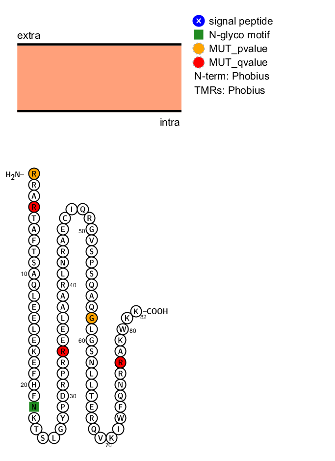
- Protter plot
> protter(lm)
A request to the Protter server is sent and a png file is downloaded with the possible sequence structure of the protein and the significant position colored in orange and red
Summary
Launch all the command we saw in one shot
> library(LowMACA)
> myBelovedFolder <- "myLowMACAOutput"
> Genes <- c("ADNP","ALX1","ALX4","ARGFX","CDX4","CRX"
			,"CUX1","CUX2","DBX2","DLX5","DMBX1","DRGX"
			,"DUXA","ESX1","EVX2","HDX","HLX","HNF1A"
			,"HOXA1","HOXA2","HOXA3","HOXA5","HOXB1","HOXB3"
			,"HOXD3","ISL1","ISX","LHX8")
> Pfam <- "PF00046"
> lm <- newLowMACA(genes=Genes , pfam=Pfam , outputFolder=myBelovedFolder)
> params(lm)$tumor_type <- c("skcm" , "stad" , "ucec" , "luad" , "lusc" , "coadread" , "brca")
> params(lm)$min_mutation_number <- 0
> lm <- setup(lm)
> lm <- entropy(lm)
> lfm(lm)
> bpAll(lm)
> lmPlot(lm)
> protter(lm)